6  When assumptions break: pleiotropy

Every estimate so far came from valid instruments, and every method landed on the truth. Real variants are not so obliging. A single variant often influences several traits at once (a phenomenon called pleiotropy), and when a variant affects the outcome through some pathway other than the exposure, it violates the exclusion restriction from Chapter 2. This chapter breaks that assumption on purpose and shows what it does to our estimates, then builds the tools that detect and resist it.

6.1 Two flavours of pleiotropy

The simulator can plant a direct variant-to-outcome effect \(\alpha_j\) on a subset of instruments. The sign of those effects matters enormously.

• Balanced. The direct effects point in random directions and roughly cancel. IVW stays approximately unbiased, because the pleiotropic pushes average out. This is the optimistic case people quietly hope holds.
• Directional. The direct effects mostly point the same way. Now they do not cancel, and they drag the estimate with them. This is the dangerous case, and the whole point of MR sensitivity analysis is to survive it.

none <- simulate_mr(pleiotropy = "none")
bal  <- simulate_mr(pleiotropy = "balanced")
dir  <- simulate_mr(pleiotropy = "directional")

6.2 Watching IVW break

Let’s run every method on all three scenarios. A small helper turns a simulated dataset into two-sample summary statistics and applies IVW, MR-Egger, and the weighted median.

analyse <- function(sim) {
  ts <- split_two_sample(sim)
  bx <- sapply(seq_len(ncol(ts$sample1$G)), \(j) snp_assoc(ts$sample1$G[, j], ts$sample1$x)["beta"])
  by <- sapply(seq_len(ncol(ts$sample2$G)), \(j) snp_assoc(ts$sample2$G[, j], ts$sample2$y)["beta"])
  sy <- sapply(seq_len(ncol(ts$sample2$G)), \(j) snp_assoc(ts$sample2$G[, j], ts$sample2$y)["se"])
  list(bx = bx, by = by, sy = sy,
       ivw = mr_ivw(bx, by, sy),
       egg = mr_egger(bx, by, sy),
       wm  = mr_weighted_median(bx, by, sy, n_boot = 1000))
}
res <- lapply(list(none = none, balanced = bal, directional = dir), analyse)

tab <- do.call(rbind, lapply(names(res), function(sc) {
  r <- res[[sc]]
  data.frame(scenario = sc,
             IVW            = round(r$ivw$estimate, 3),
             `MR-Egger`     = round(r$egg$estimate[2], 3),
             `Weighted median` = round(r$wm$estimate, 3),
             `Egger intercept` = round(r$egg$estimate[1], 4),
             check.names = FALSE)
}))
tab

	scenario	IVW	MR-Egger	Weighted median	Egger intercept
beta	none	0.357	0.314	0.371	0.0160
beta1	balanced	0.329	0.298	0.306	0.0116
beta2	directional	0.499	0.355	0.423	0.0541

Read the IVW column top to bottom. With no pleiotropy it is near 0.35. With balanced pleiotropy it holds up. With directional pleiotropy it lurches up to roughly 0.5: a large, confident, completely spurious causal effect. Nothing in the IVW estimate itself warns you; its confidence interval is happily narrow around the wrong number. This is the failure mode that makes naïve MR dangerous.

6.3 MR-Egger: let the line miss the origin

IVW forced the regression of \(\beta_Y\) on \(\beta_X\) through the origin. That constraint is precisely what directional pleiotropy exploits: if invalid variants all nudge the outcome the same way, they lift the whole cloud of points off the origin, and a through-the-origin line has to tilt to chase them.

MR-Egger (Bowden, Davey Smith, and Burgess 2015) relaxes the constraint. It fits the same weighted regression but allows an intercept:

\[ \beta_{Y_j} \;=\; \beta_0 + \theta\,\beta_{X_j} + \text{error}. \]

The payoff is twofold. The intercept \(\beta_0\) estimates the average directional pleiotropy. Under valid instruments it should be zero, so a non-zero intercept is a red flag. And the slope \(\theta\) stays consistent for the causal effect even when that intercept is non-zero, provided pleiotropy is uncorrelated with instrument strength (the “InSIDE” assumption).

print(mr_egger)

function (bx, by, sy) 
{
    s <- sign(bx)
    s[s == 0] <- 1
    bxp <- bx * s
    byp <- by * s
    w <- 1/sy^2
    X <- cbind(1, bxp)
    WX <- X * w
    b <- solve(crossprod(X, WX), crossprod(WX, byp))
    L <- length(bx)
    resid <- byp - as.vector(X %*% b)
    s2 <- sum(w * resid^2)/(L - 2)
    V <- s2 * solve(crossprod(X, WX))
    data.frame(term = c("intercept_pleiotropy", "slope_causal"), 
        estimate = as.numeric(b), se = sqrt(diag(V)), pval = 2 * 
            pt(abs(as.numeric(b)/sqrt(diag(V))), df = L - 2, 
                lower.tail = FALSE))
}
<bytecode: 0x1294eb078>

egg <- res$directional$egg
egg

	term	estimate	se	pval
	intercept_pleiotropy	0.0541385	0.0226841	0.0202865
bxp	slope_causal	0.3550584	0.0666029	0.0000017

In the directional scenario the Egger slope comes back to about 0.36, close to the true 0.35, while IVW was stuck up near 0.5. The intercept, at roughly 0.05 against essentially zero under valid instruments, is no longer null. That is the correct flag: something pleiotropic is going on.

WarningDon’t lean too hard on the intercept test

Here the intercept reaches significance, helped by having sixty instruments with a wide spread of strengths. Do not generalise from that. MR-Egger’s intercept test is notoriously underpowered with fewer variants or little variation in instrument strength, so a non-significant intercept is not reassurance that pleiotropy is absent. Read a non-zero point estimate as the warning sign, and never treat a null intercept as a clean bill of health.

6.4 The weighted median: a different kind of robustness

MR-Egger buys robustness by changing the model. The weighted median (Bowden et al. 2016) buys it by changing the summary statistic. Take all the per-variant Wald ratios, weight them, and report their weighted median instead of their weighted mean. A median ignores extreme values, so the estimate stays consistent as long as variants making up at least half the weight are valid, even if you have no idea which ones are the bad ones.

wm <- res$directional$wm
sprintf("Weighted median (directional): %.3f  (95%% CI %.3f to %.3f)",
        wm$estimate, wm$ci[1], wm$ci[2])

[1] "Weighted median (directional): 0.423  (95% CI 0.369 to 0.477)"

It lands between the badly-biased IVW and the truth. That is typical: the weighted median and MR-Egger lean on different assumptions, so they fail in different ways. When they agree, you can believe the answer; when they diverge, you have learned that the result is fragile. That agreement-or-not is the real output of a sensitivity analysis, more than any single number.

6.5 Seeing all three at once

r  <- res$directional
d  <- data.frame(bx = r$bx, by = r$by, w = 1 / r$sy^2,
                 invalid = seq_along(r$bx) %in% dir$params$invalid)
b0 <- r$egg$estimate[1]; b1 <- r$egg$estimate[2]
# egger fit was oriented on positive bx; recover display intercept/slope
ggplot(d, aes(bx, by)) +
  geom_hline(yintercept = 0, colour = mrcol("grey"), linewidth = 0.3) +
  geom_vline(xintercept = 0, colour = mrcol("grey"), linewidth = 0.3) +
  geom_abline(aes(slope = dir$params$theta, intercept = 0, colour = "Truth"),
              linetype = "22", linewidth = 0.9) +
  geom_abline(aes(slope = r$ivw$estimate, intercept = 0, colour = "IVW (through origin)"),
              linewidth = 1) +
  geom_abline(aes(slope = b1, intercept = b0, colour = "MR-Egger (free intercept)"),
              linewidth = 1) +
  geom_point(aes(size = w, shape = invalid), colour = mrcol("blue"), alpha = 0.75) +
  scale_shape_manual(values = c(`FALSE` = 16, `TRUE` = 17),
                     labels = c("valid", "pleiotropic"), name = NULL) +
  scale_size_continuous(range = c(1.5, 5), guide = "none") +
  scale_colour_manual(values = c("Truth" = mrcol("green"),
                                 "IVW (through origin)" = mrcol("red"),
                                 "MR-Egger (free intercept)" = mrcol("amber")),
                      name = NULL) +
  labs(title = "How directional pleiotropy fools IVW but not MR-Egger",
       x = "SNP → exposure association (bx)", y = "SNP → outcome association (by)") +
  theme_mr() +
  guides(colour = guide_legend(order = 1), shape = guide_legend(order = 2))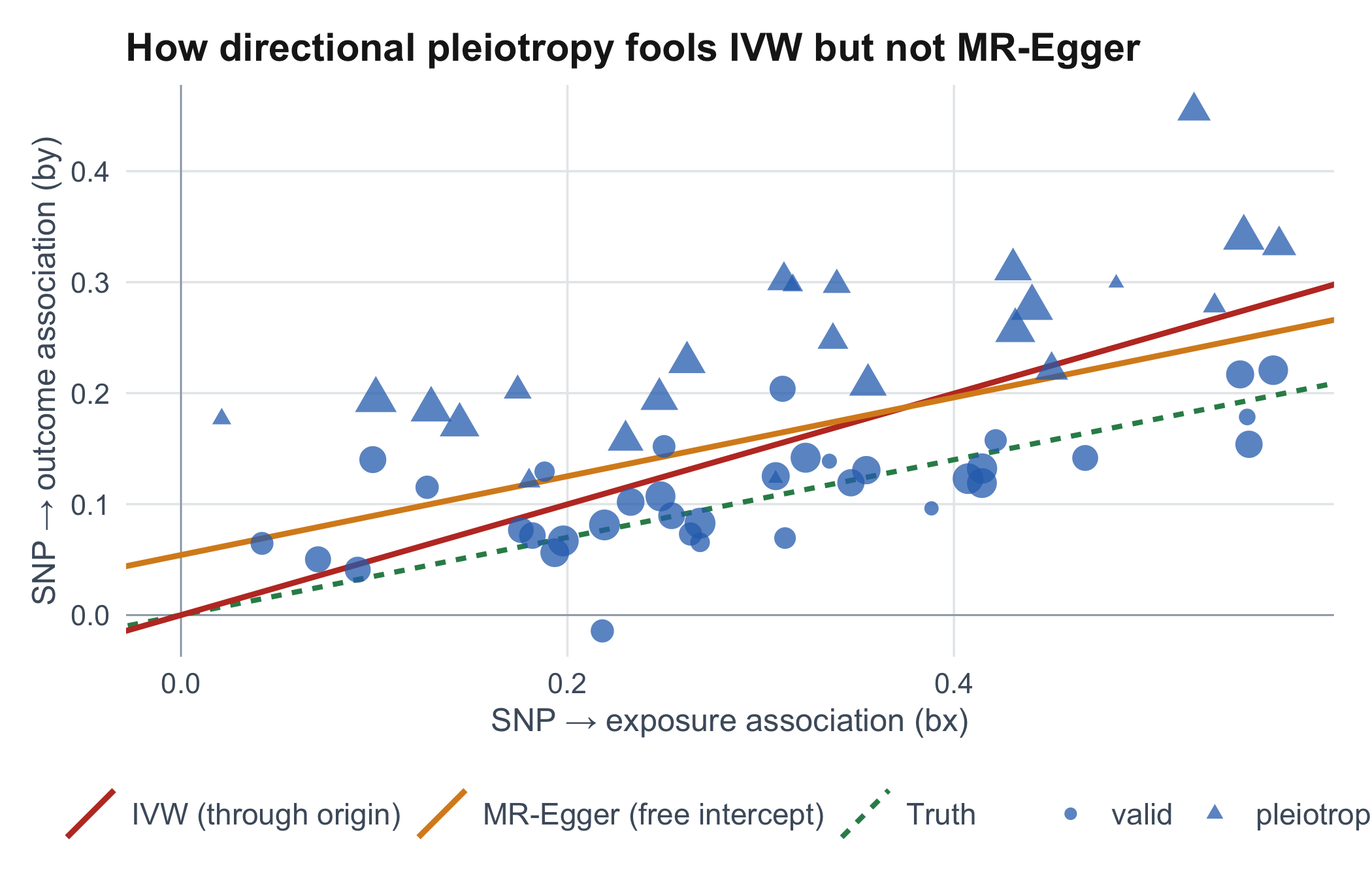

Figure 6.1: Directional pleiotropy lifts the point cloud off the origin. The through-the-origin IVW line (red) tilts up to chase it and overshoots; the MR-Egger line (amber) is free to miss the origin and its slope tracks the truth (green dashed).

6.6 Leave-one-out: is one variant driving everything?

A final, cheap diagnostic: drop each variant in turn and recompute IVW. If one variant’s removal swings the estimate, your result is hostage to that single instrument and deserves suspicion.

loo <- sapply(seq_along(r$bx), \(i) mr_ivw(r$bx[-i], r$by[-i], r$sy[-i])$estimate)
dl  <- data.frame(dropped = factor(seq_along(loo)), est = loo)
ggplot(dl, aes(est, dropped)) +
  geom_vline(xintercept = r$ivw$estimate, colour = mrcol("red"), linetype = "22") +
  geom_vline(xintercept = dir$params$theta, colour = mrcol("green"), linetype = "22") +
  geom_point(colour = mrcol("blue"), size = 1.6) +
  labs(title = "Leave-one-out IVW estimates",
       subtitle = "red = full IVW · green = truth",
       x = "IVW estimate with one variant removed", y = "Variant dropped") +
  theme_mr() +
  theme(axis.text.y = element_text(size = 6))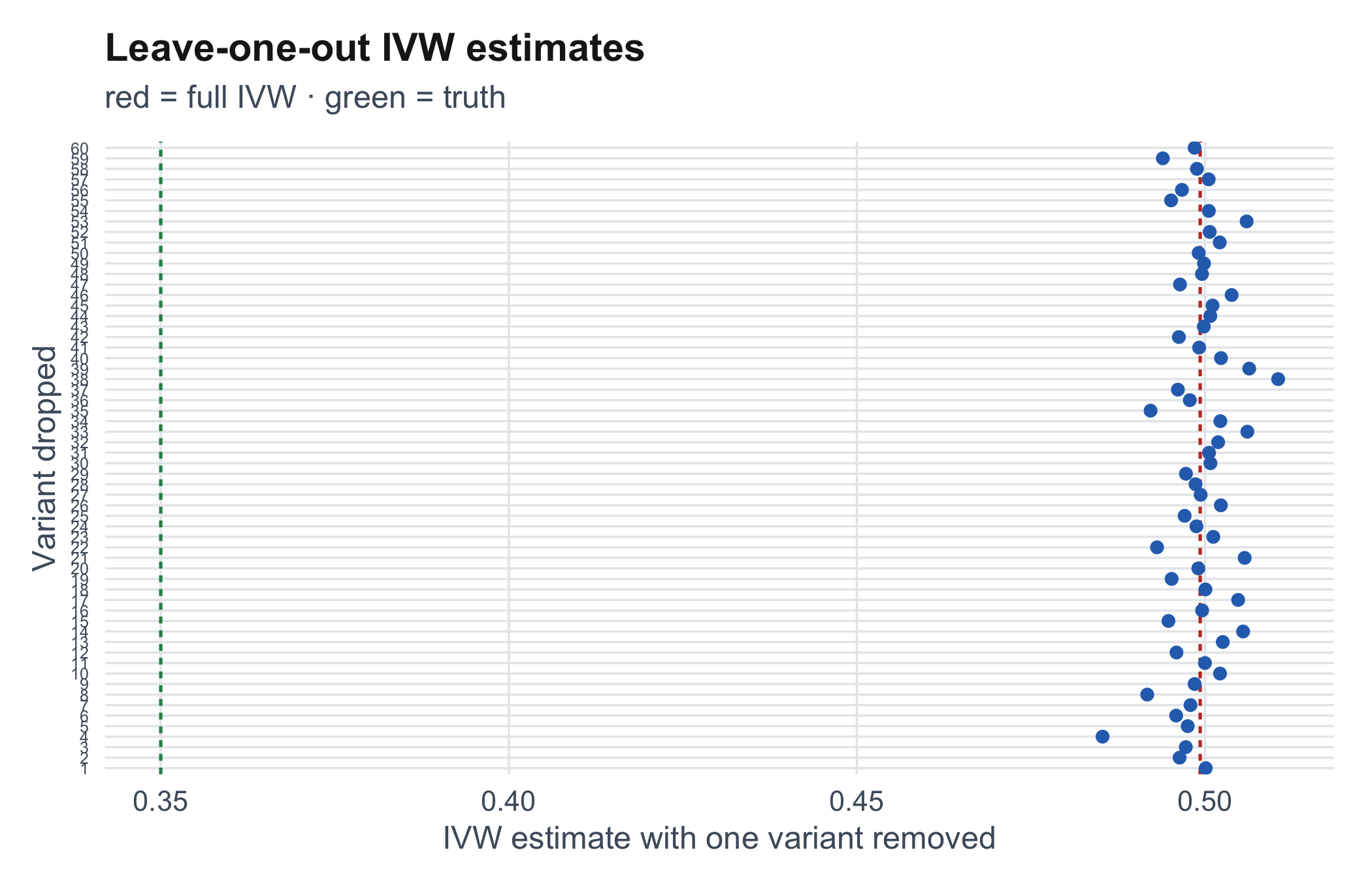

Figure 6.2: Leave-one-out IVW under directional pleiotropy. No single variant is solely responsible: the bias is spread across the pleiotropic instruments, which is exactly why it is hard to spot and why sensitivity analysis matters.

6.7 Cross-check against MendelianRandomization

library(MendelianRandomization)
obj      <- mr_input(bx = r$bx, bxse = rep(0.01, length(r$bx)), by = r$by, byse = r$sy)
pkg_egg  <- MendelianRandomization::mr_egger(obj)

data.frame(
  quantity  = c("Egger slope", "Egger intercept"),
  scratch   = round(c(r$egg$estimate[2], r$egg$estimate[1]), 4),
  package   = round(c(pkg_egg$Estimate, pkg_egg$Intercept), 4)
)

quantity	scratch	package
Egger slope	0.3551	0.3551
Egger intercept	0.0541	0.0541

The from-scratch MR-Egger matches the package on both the slope and the intercept. We have now built, and validated, the core toolkit of applied MR. Chapter 7 turns it around: how to use these ideas to read someone else’s MR paper with a critical eye.

Bowden, Jack, George Davey Smith, and Stephen Burgess. 2015. “Mendelian Randomization with Invalid Instruments: Effect Estimation and Bias Detection Through Egger Regression.” International Journal of Epidemiology 44 (2): 512–25. https://doi.org/10.1093/ije/dyv080.

Bowden, Jack, George Davey Smith, Philip C. Haycock, and Stephen Burgess. 2016. “Consistent Estimation in Mendelian Randomization with Some Invalid Instruments Using a Weighted Median Estimator.” Genetic Epidemiology 40 (4): 304–14. https://doi.org/10.1002/gepi.21965.