G_j  ~ Binomial(2, maf_j)                       # allele dosages: the instruments
U    ~ N(0, 1)                                   # unmeasured confounder
X    = sum_j bx_j * G_j + conf_x * U + noise     # exposure
Y = THETA * X + sum_j alpha_j * G_j + conf_y * U + noise # outcome3 The data: a world with a known answer
To judge an estimator honestly you need a case where you already know the right answer. Real studies never give you that. Simulation does. That makes it the natural setting for learning a method, not a compromise forced on us by data access.
The generator lives in R/simulate.R. It builds each dataset from an explicit causal model, so the true effect is whatever we say it is.
3.1 The causal model, in code
Three pieces deserve a comment. THETA is the causal effect we are hunting, fixed at 0.35. conf_x and conf_y are how strongly the confounder \(U\) leaks into the exposure and the outcome; set them to zero and the naïve regression from Chapter 1 would be correct. alpha_j is the direct effect of variant \(j\) on the outcome: the pleiotropy that breaks the exclusion restriction. When every alpha_j is zero the instruments are valid, which is the world we work in until Chapter 6.
3.2 What the variables look like
The instruments are allele dosages: each variant is coded 0, 1, or 2 copies of an allele, with frequencies drawn to resemble common variants. The exposure and outcome are continuous.
g1 <- ggplot(data.frame(g = factor(sim$G[, 1])), aes(g)) +
  geom_bar(fill = mrcol("blue"), width = 0.7, alpha = 0.9) +
  labs(title = "One instrument (rs0001)", x = "Allele dosage", y = "Individuals") +
  theme_mr()
g2 <- ggplot(data.frame(x = sim$x), aes(x)) +
  geom_histogram(bins = 40, fill = mrcol("slate"), alpha = 0.85) +
  labs(title = "The exposure X", x = "Exposure", y = "Individuals") +
  theme_mr()
g1 + g2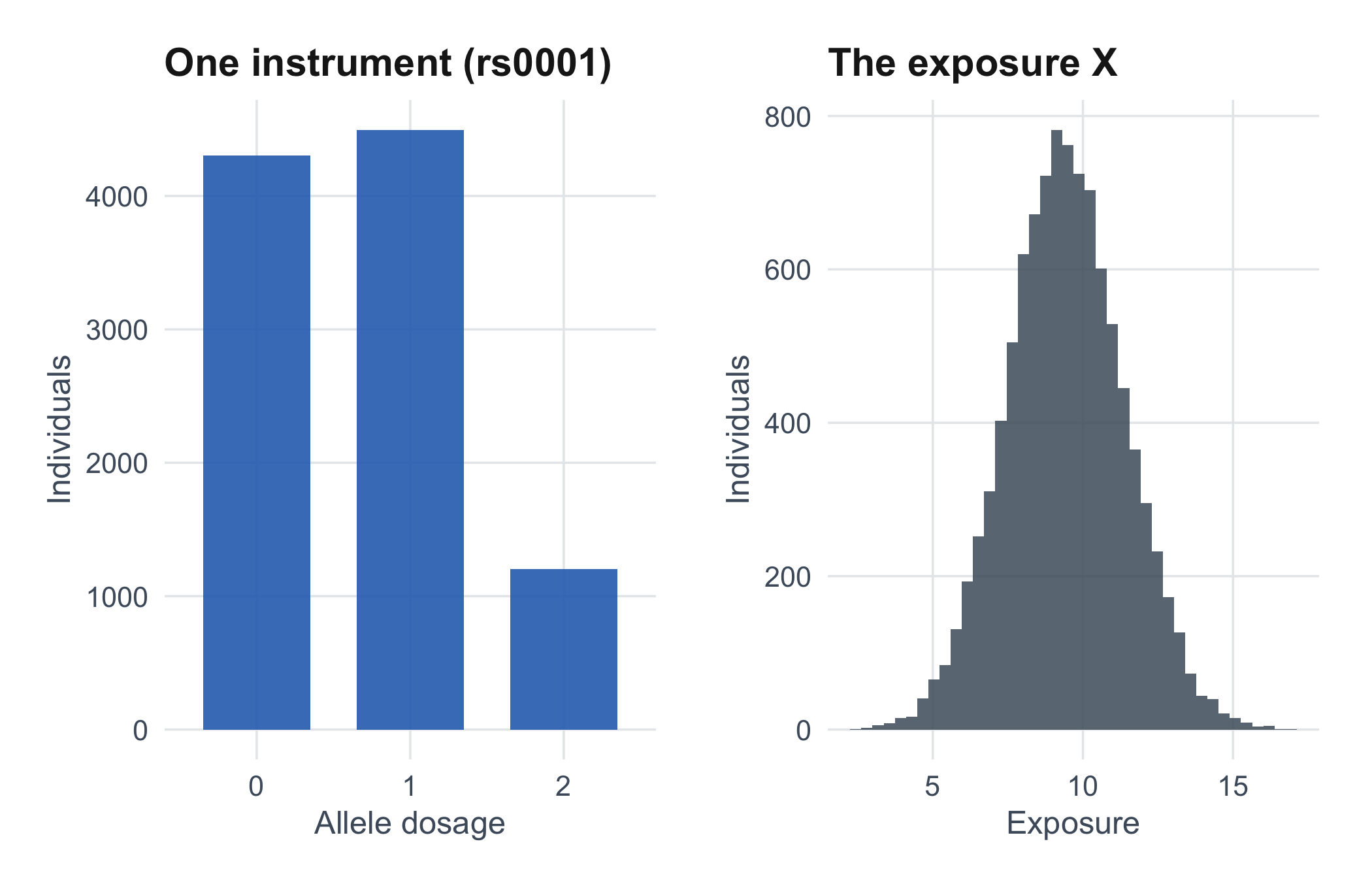
3.3 Are the instruments strong enough?
Relevance (the one assumption we can check) is usually reported as an F-statistic from regressing the exposure on the instruments. The rule of thumb is that \(F > 10\) keeps weak-instrument bias small. We can compute it directly.
[1] "Instrument F-statistic = 295.1 (rule of thumb: comfortable above 10)"[1] "The instruments jointly explain 64.0% of the variance in the exposure."An F well past 10 means these variants move the exposure decisively, so the ratios we build in later chapters rest on solid denominators. Weak instruments are one of the classic ways MR goes wrong, and it is reassuring to rule the problem out before going further.
3.4 The two shapes the data comes in
MR is done in two settings, and the rest of the book follows that split.
- One-sample. Individual-level records for exposure, outcome, and genotype, all on the same people. This is Chapter 4, where we run two-stage least squares.
- Two-sample. You never see individuals, only summary statistics: for each variant, its association with the exposure (from one study) and with the outcome (from another). This is how most published MR is done, because the summary numbers are freely shared while the raw data are not. Chapters 5 and 6 live here.
We can manufacture the summary-statistic form from our individual data by regressing each trait on each variant, one variant at a time. That is what summarise_snps() does.
ss <- summarise_snps(sim$G, sim$x, sim$y)
head(ss, 5)| snp | bx | sx | by | sy | |
|---|---|---|---|---|---|
| beta | rs0001 | 0.2299716 | 0.0289360 | 0.0876550 | 0.0212258 |
| beta1 | rs0002 | 0.3128183 | 0.0301328 | 0.1002602 | 0.0221489 |
| beta2 | rs0003 | 0.1790455 | 0.0387234 | 0.0312247 | 0.0283686 |
| beta3 | rs0004 | 0.5549845 | 0.0339791 | 0.1703367 | 0.0251398 |
| beta4 | rs0005 | 0.3612507 | 0.0301488 | 0.1019630 | 0.0221991 |
Each row is one variant: bx is its effect on the exposure, by its effect on the outcome, with standard errors. Everything from here on is built out of these two columns. On to the estimators, starting with the individual-level workhorse: two-stage least squares.