sim <- simulate_mr(pleiotropy = "none")   # valid instruments; confounding present
cat("True causal effect theta =", sim$params$theta, "\n")
True causal effect theta = 0.35 Here is the situation an epidemiologist faces constantly. We have an exposure \(X\) (a biomarker, a behaviour, a drug level) and an outcome \(Y\), some disease. In the data, higher \(X\) goes with higher \(Y\). The clinical question is whether pushing \(X\) down would push \(Y\) down. That is a question about a causal effect, and it is not the same question as “are \(X\) and \(Y\) correlated?”
The reason the two come apart is confounding. If some third factor \(U\) raises both \(X\) and \(Y\), then \(X\) and \(Y\) will move together even if \(X\) does nothing to \(Y\) at all. Socioeconomic status, general health, and countless unmeasured habits all play the role of \(U\) in real studies, and no amount of extra observational data makes them go away.
We can see the problem cleanly by building a world where we know the truth. In the simulator used throughout this book, the outcome is generated as
\[ Y = \theta\, X + \gamma\, U + \varepsilon, \]
with the true causal effect fixed at \(\theta = 0.35\). A confounder \(U\) feeds into both \(X\) and \(Y\). Because we wrote the model, we know the answer we are trying to recover.
sim <- simulate_mr(pleiotropy = "none") # valid instruments; confounding present
cat("True causal effect theta =", sim$params$theta, "\n")True causal effect theta = 0.35 The obvious thing to do is regress \(Y\) on \(X\). The hand-written naive_ols() in R/mr_estimators.R does exactly that.
ols <- naive_ols(sim$x, sim$y)
sprintf("naive OLS estimate: %.3f  (95%% CI %.3f to %.3f)",
        ols$estimate, ols$ci[1], ols$ci[2])
[1] "naive OLS estimate: 0.443 (95% CI 0.432 to 0.455)"The estimate lands clearly above the true 0.35, and the confidence interval does not come close to covering it. The regression is not noisy. It is confidently, systematically wrong. It is measuring the causal effect plus the confounding, and it has no way to tell you which is which.
d <- data.frame(x = sim$x, y = sim$y)
ggplot(d, aes(x, y)) +
  geom_point(alpha = 0.12, colour = mrcol("grey"), size = 0.7) +
  geom_abline(aes(slope = ols$estimate, intercept = mean(sim$y) - ols$estimate * mean(sim$x),
                  colour = "Observational (OLS)"), linewidth = 1.1) +
  geom_abline(aes(slope = sim$params$theta,
                  intercept = mean(sim$y) - sim$params$theta * mean(sim$x),
                  colour = "True causal effect"), linewidth = 1.1, linetype = "22") +
  scale_colour_manual(values = c("Observational (OLS)" = mrcol("red"),
                                 "True causal effect"  = mrcol("green")),
                      name = NULL) +
  labs(title = "The observational slope is not the causal slope",
       x = "Exposure X", y = "Outcome Y") +
  theme_mr()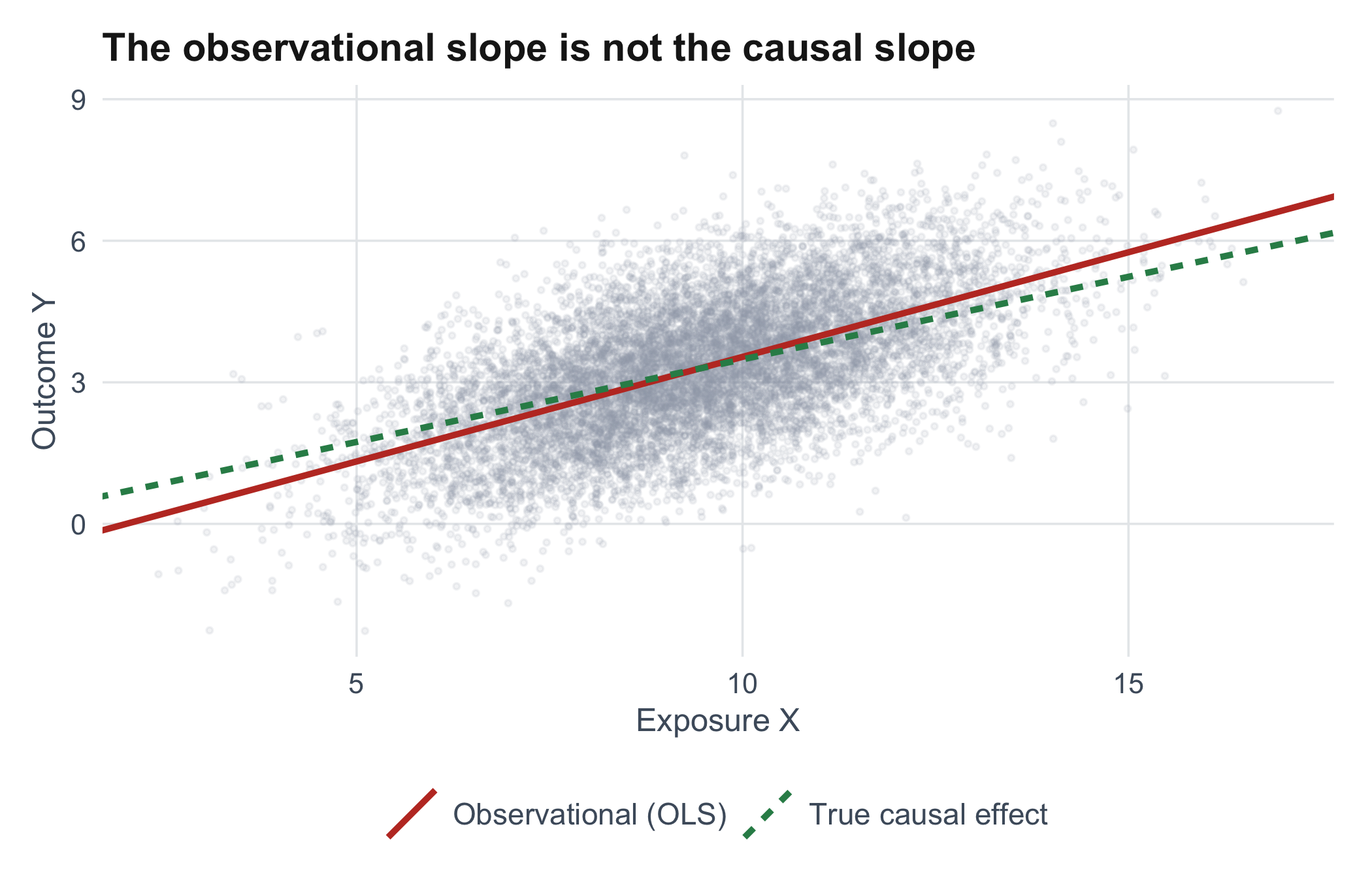
Adjusting for confounders you can measure helps only with the confounders you can measure. The ones you cannot (in most health data, that is most of them) remain. This is the wall that observational epidemiology keeps running into.
Mendelian randomisation gets around the wall instead of climbing it. Instead of modelling the confounding, it finds a source of variation in \(X\) that is disconnected from \(U\) to begin with: the genetic variants a person happened to inherit. The next chapter explains why inheritance can stand in for randomisation, and what has to be true for the trick to work.