4  One-sample MR: two-stage least squares

When you hold individual-level data (exposure, outcome, and genotype on the same people), the classic instrumental-variable estimator is two-stage least squares (2SLS). Its name is also its recipe, and the recipe is short enough to write out in full.

sim <- simulate_mr(pleiotropy = "none")   # valid instruments, true theta = 0.35

4.1 The recipe

Stage 1. Regress the exposure on the instruments and keep the fitted values \(\hat X\). These fitted values are the part of the exposure that the genetics explains, and only that part. Whatever the confounder \(U\) contributed to \(X\) is left behind in the residuals, because the variants are independent of \(U\).

Stage 2. Regress the outcome on \(\hat X\). Since \(\hat X\) is scrubbed of confounding, its slope is an estimate of the causal effect, not the causal effect plus contamination.

That is the whole idea: launder the exposure through the instruments so that only its randomised component survives, then use that clean component to predict the outcome. Here it is in base R, straight from R/mr_estimators.R:

print(tsls)

function (G, x, y) 
{
    n <- length(y)
    Z <- cbind(1, G)
    b1 <- solve(crossprod(Z), crossprod(Z, x))
    xhat <- as.vector(Z %*% b1)
    Dhat <- cbind(1, xhat)
    b2 <- solve(crossprod(Dhat), crossprod(Dhat, y))
    theta <- b2[2]
    Dact <- cbind(1, x)
    resid <- y - as.vector(Dact %*% b2)
    s2 <- sum(resid^2)/(n - 2)
    V <- s2 * solve(crossprod(Dhat))
    se <- sqrt(V[2, 2])
    list(estimate = as.numeric(theta), se = as.numeric(se), ci = as.numeric(theta) + 
        c(-1.96, 1.96) * as.numeric(se))
}

The one subtlety worth flagging is the standard error. The residuals are computed from the actual exposure, not the fitted \(\hat X\). That is the correct structural-equation variance, and it is what a proper IV routine returns. Getting this detail right is exactly why it is worth writing the estimator once by hand before trusting a package.

4.2 Running it

ols <- naive_ols(sim$x, sim$y)
iv  <- tsls(sim$G, sim$x, sim$y)

results <- rbind(
  mr_row("Truth (planted)", list(estimate = sim$params$theta, se = NA,
                                  ci = c(NA, NA))),
  mr_row("Naive OLS",       ols),
  mr_row("2SLS (from scratch)", iv)
)
results

method	estimate	se	ci_low	ci_high
Truth (planted)	0.350	NA	NA	NA
Naive OLS	0.443	0.006	0.432	0.455
2SLS (from scratch)	0.351	0.007	0.337	0.366

The naïve estimate sits up at 0.44, inflated by confounding. Two-stage least squares pulls it back to 0.35, right on top of the true 0.35, and its confidence interval covers the truth. Same data, same outcome, but by routing through the instruments we recovered the causal effect the ordinary regression could not.

plt <- results[!is.na(results$se), ]
plt$method <- factor(plt$method, levels = rev(plt$method))
ggplot(plt, aes(estimate, method)) +
  geom_vline(xintercept = sim$params$theta, linetype = "22", colour = mrcol("green"), linewidth = 0.9) +
  geom_errorbarh(aes(xmin = ci_low, xmax = ci_high), height = 0.18, colour = mrcol("slate")) +
  geom_point(size = 3, colour = mrcol("blue")) +
  annotate("text", x = sim$params$theta, y = 2.5, label = "  truth", hjust = 0,
           colour = mrcol("green"), size = 3.4) +
  labs(title = "Naive regression vs two-stage least squares",
       x = "Estimated causal effect of X on Y", y = NULL) +
  theme_mr()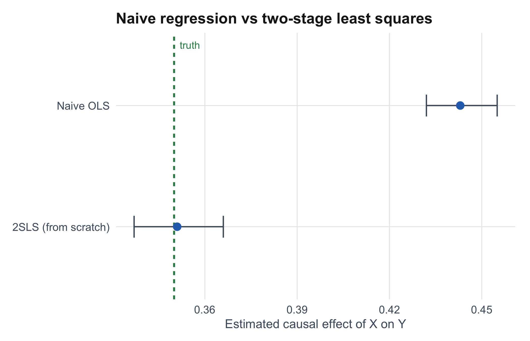

Figure 4.1: The naïve estimate misses the planted truth; 2SLS lands on it. Bars are 95% confidence intervals.

4.3 Checking our work against ivreg

Writing an estimator from scratch is only convincing if it agrees with a trusted implementation. The ivreg package fits exactly this model with the formula syntax outcome ~ exposure | instruments.

library(ivreg)
df   <- data.frame(y = sim$y, x = sim$x, sim$G)
inst <- paste(colnames(sim$G), collapse = " + ")
m    <- ivreg(as.formula(paste("y ~ x |", inst)), data = df)
co   <- summary(m)$coefficients["x", ]

data.frame(
  source   = c("tsls() from scratch", "ivreg package"),
  estimate = round(c(iv$estimate, co["Estimate"]), 4),
  se       = round(c(iv$se, co["Std. Error"]), 4)
)

	source	estimate	se
	tsls() from scratch	0.3514	0.0074
Estimate	ivreg package	0.3514	0.0074

The point estimate and the standard error match to four decimal places. The hand-written function is not an approximation to the package; it is the same computation, and now you have seen every line of it.

4.4 What one-sample MR cannot do for you

2SLS is clean when you have everyone’s records. But it also inherits a soft spot: with individual data, if the instruments are weak the estimate is biased toward the confounded observational value, which is the worst possible direction to be pulled. And in practice you rarely have one cohort measured for both the exposure and the outcome anyway. Published MR gets around both problems by working from summary statistics drawn from two different studies. That is Chapter 5.