Most MR you read in journals never touches individual records. Instead it uses two sets of summary statistics: from one study, how each variant associates with the exposure; from another, how each variant associates with the outcome. This is the two-sample design, and it is popular for a practical reason: those per-variant numbers are published in consortium GWAS, while the raw data stay locked down.
We can recreate the setting by splitting our simulated cohort in half and computing associations separately in each half, so no individual contributes to both sides.
   Min. 1st Qu.  Median    Mean 3rd Qu.    Max.
-0.0966  0.2926  0.3740  0.3971  0.4454  1.9678
The individual guesses scatter around, some tighter than others. The job of an MR estimator is to combine them into one number, giving more say to the variants that carry more information.
5.2 Combining them: inverse-variance weighting
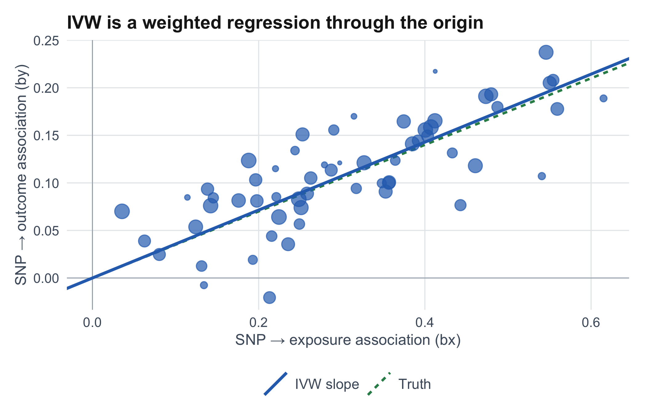
The inverse-variance weighted (IVW) estimate (Burgess, Butterworth, and Thompson 2013) is a weighted average of the Wald ratios, with each variant weighted by how precise its outcome association is (weight \(= 1/\text{se}_{Y}^2\)). Equivalently (and this is the more useful way to see it), IVW is a weighted linear regression of the outcome associations on the exposure associations, forced through the origin:
The slope of that line is the causal effect. The regression goes through the origin because a variant with no effect on the exposure should, under valid assumptions, have no effect on the outcome either.
function (bx, by, sy, random = TRUE)
{
    w <- 1/sy^2
    theta <- sum(w * bx * by)/sum(w * bx^2)
    se_fe <- sqrt(1/sum(w * bx^2))
    L <- length(bx)
    resid <- by - theta * bx
    Q <- sum(w * resid^2)
    phi <- if (random)
        max(1, Q/(L - 1))
    else 1
    se <- se_fe * sqrt(phi)
    list(estimate = theta, se = se, ci = theta + c(-1.96, 1.96) *
        se, Q = Q, df = L - 1, Q_pval = pchisq(Q, L - 1, lower.tail = FALSE))
}
ivw<-mr_ivw(bx, by, sy)sprintf("IVW estimate: %.3f (95%% CI %.3f to %.3f). Truth = %.2f",ivw$estimate, ivw$ci[1], ivw$ci[2], sim$params$theta)
[1] "IVW estimate: 0.357 (95% CI 0.331 to 0.384). Truth = 0.35"
The estimate recovers the planted 0.35 from nothing but the two columns of associations, without ever seeing a single individual.
d<-data.frame(bx =bx, by =by, w =1/sy^2)ggplot(d, aes(bx, by))+geom_hline(yintercept =0, colour =mrcol("grey"), linewidth =0.3)+geom_vline(xintercept =0, colour =mrcol("grey"), linewidth =0.3)+geom_abline(aes(slope =sim$params$theta, intercept =0, colour ="Truth"), linetype ="22", linewidth =0.9)+geom_abline(aes(slope =ivw$estimate, intercept =0, colour ="IVW slope"), linewidth =1.1)+geom_point(aes(size =w), colour =mrcol("blue"), alpha =0.7)+scale_size_continuous(range =c(1, 5), guide ="none")+scale_colour_manual(values =c("Truth"=mrcol("green"), "IVW slope"=mrcol("blue")), name =NULL)+labs(title ="IVW is a weighted regression through the origin", x ="SNP → exposure association (bx)", y ="SNP → outcome association (by)")+theme_mr()
Figure 5.1: Each point is one variant, placed by its exposure association (x) and outcome association (y). Point size reflects its weight. The IVW slope through the origin is the causal effect, and it recovers the truth.
5.3 Fixed versus random effects
The variants do not all agree; that disagreement is heterogeneity, and Cochran’s \(Q\) measures it. When the ratios scatter more than their standard errors alone would predict, some instruments are probably doing something extra: a hint of the pleiotropy we tackle next. The mr_ivw() function inflates its standard error by the overdispersion (a random-effects correction) so the interval is not falsely narrow.
With valid instruments there is little heterogeneity and nothing to worry about. Hold that \(Q\) in mind, though: in Chapter 6 we deliberately break the exclusion restriction, watch IVW sail confidently off to the wrong answer, and build the diagnostics that catch it.
5.4 Cross-check against MendelianRandomization
library(MendelianRandomization)obj<-mr_input(bx =bx, bxse =rep(0.01, length(bx)), by =by, byse =sy)pkg_ivw<-MendelianRandomization::mr_ivw(obj)data.frame( source =c("mr_ivw() from scratch", "MendelianRandomization pkg"), estimate =round(c(ivw$estimate, pkg_ivw$Estimate), 4))
source
estimate
mr_ivw() from scratch
0.3572
MendelianRandomization pkg
0.3572
Same answer. The hand-written weighted regression is doing exactly what the established package does.
Burgess, Stephen, Adam Butterworth, and Simon G. Thompson. 2013. “Mendelian Randomization Analysis with Multiple Genetic Variants Using Summarized Data.”Genetic Epidemiology 37 (7): 658–65. https://doi.org/10.1002/gepi.21758.
Source Code
# Two-sample MR: inverse-variance weighting```{r}#| label: setup#| include: falsesource("R/theme_mr.R")source("R/simulate.R")source("R/mr_estimators.R")library(ggplot2)```Most MR you read in journals never touches individual records. Instead it uses two sets of **summary statistics**: from one study, how each variant associates with the exposure; from another, how each variant associates with the outcome. This is the *two-sample* design, and it is popular for a practical reason: those per-variant numbers are published in consortium GWAS, while the raw data stay locked down.We can recreate the setting by splitting our simulated cohort in half and computing associations separately in each half, so no individual contributes to both sides.```{r}#| label: two-sample-splitsim <-simulate_mr(pleiotropy ="none")ts <-split_two_sample(sim)bx <-sapply(seq_len(ncol(ts$sample1$G)), \(j) snp_assoc(ts$sample1$G[, j], ts$sample1$x)["beta"])by <-sapply(seq_len(ncol(ts$sample2$G)), \(j) snp_assoc(ts$sample2$G[, j], ts$sample2$y)["beta"])sy <-sapply(seq_len(ncol(ts$sample2$G)), \(j) snp_assoc(ts$sample2$G[, j], ts$sample2$y)["se"])head(data.frame(bx, by, sy), 4)```## One instrument at a time: the Wald ratioRecall the atom from Chapter 2. For a single variant, the causal effect estimate is its outcome association divided by its exposure association:$$\hat\theta_j \;=\; \frac{\beta_{Y_j}}{\beta_{X_j}}.$$Each variant gives its own noisy guess at the same underlying effect.```{r}#| label: waldwr <-wald_ratio(bx, by, sy)summary(wr$estimate)```The individual guesses scatter around, some tighter than others. The job of an MR estimator is to combine them into one number, giving more say to the variants that carry more information.## Combining them: inverse-variance weightingThe **inverse-variance weighted (IVW)** estimate [@burgess2013] is a weighted average of the Wald ratios, with each variant weighted by how precise its outcome association is (weight $= 1/\text{se}_{Y}^2$). Equivalently (and this is the more useful way to see it), IVW is a weighted linear regression of the outcome associations on the exposure associations, *forced through the origin*:$$\beta_{Y_j} \;=\; \theta\,\beta_{X_j} + \text{error}, \qquad \text{weights } 1/\text{se}_{Y_j}^2 .$$The slope of that line is the causal effect. The regression goes through the origin because a variant with no effect on the exposure should, under valid assumptions, have no effect on the outcome either.```{r}#| label: show-ivwprint(mr_ivw)``````{r}#| label: run-ivwivw <-mr_ivw(bx, by, sy)sprintf("IVW estimate: %.3f (95%% CI %.3f to %.3f). Truth = %.2f", ivw$estimate, ivw$ci[1], ivw$ci[2], sim$params$theta)```The estimate recovers the planted `r TRUE_THETA` from nothing but the two columns of associations, without ever seeing a single individual.```{r}#| label: fig-ivw#| fig-cap: "Each point is one variant, placed by its exposure association (x) and outcome association (y). Point size reflects its weight. The IVW slope through the origin is the causal effect, and it recovers the truth."d <-data.frame(bx = bx, by = by, w =1/ sy^2)ggplot(d, aes(bx, by)) +geom_hline(yintercept =0, colour =mrcol("grey"), linewidth =0.3) +geom_vline(xintercept =0, colour =mrcol("grey"), linewidth =0.3) +geom_abline(aes(slope = sim$params$theta, intercept =0, colour ="Truth"),linetype ="22", linewidth =0.9) +geom_abline(aes(slope = ivw$estimate, intercept =0, colour ="IVW slope"),linewidth =1.1) +geom_point(aes(size = w), colour =mrcol("blue"), alpha =0.7) +scale_size_continuous(range =c(1, 5), guide ="none") +scale_colour_manual(values =c("Truth"=mrcol("green"), "IVW slope"=mrcol("blue")),name =NULL) +labs(title ="IVW is a weighted regression through the origin",x ="SNP → exposure association (bx)", y ="SNP → outcome association (by)") +theme_mr()```## Fixed versus random effectsThe variants do not all agree; that disagreement is **heterogeneity**, and Cochran's $Q$ measures it. When the ratios scatter more than their standard errors alone would predict, some instruments are probably doing something extra: a hint of the pleiotropy we tackle next. The `mr_ivw()` function inflates its standard error by the overdispersion (a random-effects correction) so the interval is not falsely narrow.```{r}#| label: hetsprintf("Cochran's Q = %.1f on %d df (p = %.3f)", ivw$Q, ivw$df, ivw$Q_pval)```With valid instruments there is little heterogeneity and nothing to worry about. Hold that $Q$ in mind, though: in [Chapter 6](06-when-assumptions-break.qmd) we deliberately break the exclusion restriction, watch IVW sail confidently off to the wrong answer, and build the diagnostics that catch it.## Cross-check against `MendelianRandomization````{r}#| label: pkg-checklibrary(MendelianRandomization)obj <-mr_input(bx = bx, bxse =rep(0.01, length(bx)), by = by, byse = sy)pkg_ivw <- MendelianRandomization::mr_ivw(obj)data.frame(source =c("mr_ivw() from scratch", "MendelianRandomization pkg"),estimate =round(c(ivw$estimate, pkg_ivw$Estimate), 4))```Same answer. The hand-written weighted regression is doing exactly what the established package does.