calibrationfunction (label, score, eps = 1e-06)
{
s <- pmin(pmax(score, eps), 1 - eps)
fit <- glm(label ~ qlogis(s), family = binomial())
c(intercept = unname(coef(fit)[1]), slope = unname(coef(fit)[2]))
}
<bytecode: 0x113db4988>Chapter 4 established that AUROC cannot see the numbers, only their order. This chapter asks the question it cannot answer: when the model says 0.8, does the event happen 80% of the time?
The calibration slope regresses the outcome on the logit of the predicted probability. Perfect calibration gives slope 1, intercept 0. Slope below 1 means predictions are too extreme; above 1, too conservative.
calibrationfunction (label, score, eps = 1e-06)
{
s <- pmin(pmax(score, eps), 1 - eps)
fit <- glm(label ~ qlogis(s), family = binomial())
c(intercept = unname(coef(fit)[1]), slope = unname(coef(fit)[2]))
}
<bytecode: 0x113db4988>Expected calibration error bins the predictions and averages the absolute gap between predicted and observed rates within each bin. It is the metric most commonly reported in the machine-learning literature.
ecefunction (label, score, n_bins = 10L)
{
bins <- cut(score, breaks = seq(0, 1, length.out = n_bins +
1L), include.lowest = TRUE)
parts <- tapply(seq_along(label), bins, function(ix) {
if (length(ix) == 0L)
return(0)
(length(ix)/length(label)) * abs(mean(label[ix]) - mean(score[ix]))
})
sum(unlist(parts), na.rm = TRUE)
}
<bytecode: 0x10da89b28>Both are reasonable. On this data they disagree completely.
| Group | Calibration slope | ECE | Brier | AUROC |
|---|---|---|---|---|
| overall | 1.595 | 0.351 | 0.246 | 0.867 |
| I-II | 1.849 | 0.355 | 0.241 | 0.897 |
| III-IV | 1.501 | 0.356 | 0.251 | 0.855 |
| V-VI | 0.502 | 0.293 | 0.265 | 0.655 |
The slope says V-VI is badly miscalibrated: 0.50 against 1.85 in I-II. These are opposite failures: predictions too extreme in one group, too conservative in the other. Pooled, they average to 1.60, a number describing no one in the dataset.
ECE says all three groups are the same, to within 0.06.
ECE takes an absolute value inside each bin. Systematic over-prediction in one part of the score range and under-prediction in another therefore contribute in the same direction, and the tilt in the whole relationship never shows up. It measures how far off predictions are, not in which direction, systematically.
The slope, being a regression coefficient, sees the tilt directly.
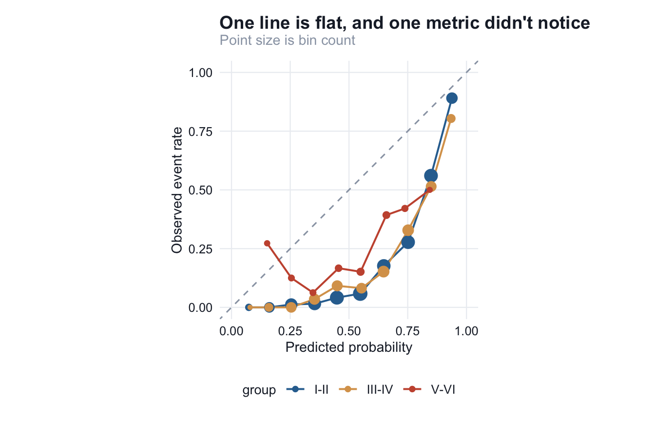
The V-VI line is visibly flatter than the diagonal: as the model’s confidence rises, the observed rate barely follows. That is a slope of 0.5, drawn.
If the model feeds a ranked worklist, miscalibration is survivable, because order is preserved. If it feeds a threshold, it is not. A referral rule of “investigate if p > 0.7” assumes 0.7 means the same thing in every patient. Here it does not, and the group where it means least is the group already least likely to have been examined by a specialist.
This is the standard signature of a transported model, and it is why calibration is the first thing to break and the last thing to be reported (1). TRIPOD+AI now asks for calibration to be reported explicitly, with a plot, for exactly this reason (2).
The slope and intercept catch systematic tilt; ECE catches local wobble; the plot catches things neither summarises. Anyone reporting a single calibration number is choosing which failures they are willing to miss.