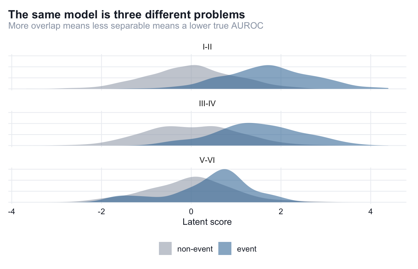
To trust a measuring instrument, you calibrate it against something whose length you already know. Real evaluation data can never be that reference, because with real data the truth (the model’s actual discrimination in each subgroup) is precisely what you are trying to estimate and never get to see. So we simulate, and we simulate in a way that hands us the answer up front.
The three strata
The separations and sizes are chosen to caricature a common situation: a model that is sharp in the group that dominates the data and dull in the group that does not. The small group is also the one where the signal is genuinely weaker.
| I-II |
1800 |
1.75 |
0.892 |
| III-IV |
900 |
1.45 |
0.847 |
| V-VI |
160 |
0.80 |
0.714 |
Two things are held fixed on purpose. The prevalence is the same 0.22 in every stratum, so that no performance gap can later be blamed on a difference in base rates. The gap will be about separation and sample size, nothing else. And the seed is fixed, so every number in this book is reproducible to the digit.
In I-II the two distributions barely touch; in V-VI they sit almost on top of each other. That overlap is the true AUROC of 0.714, drawn.
The score column the rest of the book uses is just this latent value squeezed through plogis() onto the 0–1 probability scale: a stand-in for a model that is imperfectly calibrated, which becomes the subject of Chapter 6. Everything downstream reads only label and score, exactly as it would for a real model’s output.
With a world whose answer we know, we can now write an estimator and prove it recovers that answer.