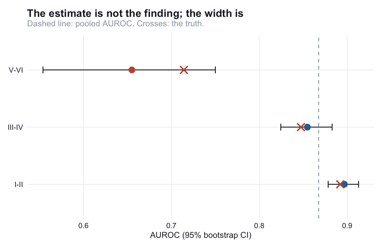
# Uncertainty is the finding
```{r}
#| include: false
source("../R/simulate.R"); source("../R/metrics.R"); source("../R/theme_eval.R")
df <- simulate_predictions()
rep <- stratified_report(df, n_boot = 2000L)
tt <- truth_table()
```
Chapter 4 produced an estimate of 0.655 in the smallest stratum against a
truth of 0.714. The question this chapter answers is whether that discrepancy
was detectable and, more usefully, whether the study could have detected
anything at all.
## The stratified bootstrap
Resample with replacement, recompute, repeat, take percentiles. The only
subtlety worth caring about is that resampling is done **within outcome
class**:
```{r}
boot_ci
```
Resampling rows without regard to outcome regularly produces, in a stratum of
39 events, replicates containing no events at all. The metric is then
undefined, those replicates get quietly dropped, and the interval becomes a
statement about which replicates happened to survive. Stratifying fixes it.
## What the intervals look like
```{r}
#| echo: false
rep$true_auroc <- c(NA, tt$true_auroc[match(rep$group[-1], tt$group)])
knitr::kable(
rep[, c("group","n","events","true_auroc","auroc","auroc_lo","auroc_hi","ci_width")],
digits = 3, col.names = c("Group","n","Events","True","Estimate","Lower","Upper","Width")
)
```
```{r}
#| echo: false
#| fig-cap: "Subgroup AUROC with 95% bootstrap intervals. Crosses mark the planted truth."
d <- rep[rep$group != "__overall__", ]
ggplot(d, aes(y = group)) +
geom_vline(xintercept = rep$auroc[1], linetype = "dashed", colour = EVAL_GREY) +
geom_errorbarh(aes(xmin = auroc_lo, xmax = auroc_hi), height = 0.12,
colour = EVAL_INK) +
geom_point(aes(x = auroc, colour = underpowered), size = 3.4) +
geom_point(aes(x = true_auroc), shape = 4, size = 3.4, stroke = 1.3,
colour = EVAL_WARN) +
scale_colour_manual(values = c("FALSE" = EVAL_ACCENT, "TRUE" = EVAL_WARN),
guide = "none") +
labs(title = "The estimate is not the finding; the width is",
subtitle = "Dashed line: pooled AUROC. Crosses: the truth.",
x = "AUROC (95% bootstrap CI)", y = NULL) +
theme_eval()
```
The interval in `V-VI` is **0.196 wide**, six times the pooled interval. It
spans from "barely better than chance" to "clinically respectable". Reported
as "AUROC 0.66 in Fitzpatrick V–VI", which is how it would appear in a table,
that estimate conveys a precision it does not have.
## The gap you cannot see is the moderate one
The natural conclusion is that the smallest group is the problem. The more
useful conclusion is about the middle row. How many events would each
comparison need?
```{r}
base <- tt$true_auroc[tt$group == "I-II"]
data.frame(
  group        = c("III-IV", "V-VI"),
  true_gap     = round(base - tt$true_auroc[match(c("III-IV","V-VI"), tt$group)], 3),
  events_need  = sapply(c("III-IV","V-VI"), function(g)
                   n_events_for_gap(base, tt$true_auroc[tt$group == g])),
  events_have  = rep$events[match(c("III-IV","V-VI"), rep$group)]
)
```
The dramatic gap in `V-VI` is, just barely, detectable: 39 events against
roughly 40 required. The moderate 0.045 gap in `III-IV` needs about **445
events per group** and the data contain 181.
So the real gap in `III-IV` will be found "not statistically significant",
and reported as reassurance. This is the failure mode that matters, because
moderate gaps are the common ones, and the study is systematically blind to
exactly the range of effects most likely to exist.
::: {.callout-warning}
## "No significant difference between subgroups" is not a finding
It is the expected result of an underpowered comparison, and subgroup
comparisons are nearly always underpowered. The honest report states the
smallest gap the analysis could have detected, then says whether it detected
it. Absence of evidence, as usual, is doing no work here.
:::
## The bootstrap is not free either
The intervals above are percentile intervals, which are known to undercover
in small samples [@efron1987]. So measure it. Simulate 200 fresh datasets and
count how often the nominal 95% interval actually contains the truth:
```{r}
#| cache: true
covered <- 0; n_rep <- 200
truth <- true_auroc(GROUPS[["V-VI"]]$d)
for (r in seq_len(n_rep)) {
  set.seed(10000 + r)
  y <- rbinom(160, 1, PREVALENCE)
  s <- plogis(rnorm(160, mean = y * GROUPS[["V-VI"]]$d, sd = 1))
  ci <- boot_ci(y, s, auroc, n_boot = 400L, seed = r)
  if (!is.na(ci[["lower"]]) && truth >= ci[["lower"]] && truth <= ci[["upper"]])
    covered <- covered + 1
}
covered / n_rep
```
**89.5%, not 95%.** The intervals in this chapter are, if anything, too
narrow, which strengthens the argument. BCa intervals or the analytic
Hanley–McNeil variance [@hanley1982] would be the next step.